Nice set of 3 videos to teach Structural Unemployment due to technological change. Where did the jobs go? Oh, I see now...

When teaching Structural Unemployment it is quite common for teachers to use the auto manufacturing sector as a prime example of how advancements in technology reduce the need for assembly line workers.

I am not sure students today, who are used to technology and likely do not have parents who work on an assembly line, understand how significant the changes have been over just the past 100 years.

Here are a series of 3 videos that show the progression of technology and processes that went into making vehicles.

I find the one from 1936 the most intriguing.  I was surprised by the high level of mechanical engineering in the technology used on the assembly line.

It is interesting to compare/contrast the levels of employment you see in each of the time periods and the tasks that people performed.  You can vividly see how jobs were automated out of existence over time.

Very early 1900's:

From 1936:

Very recent video of a BMW facility (I think in Spartenburg, South Carolina)

Latest numbers on the National Debt in nice pie chart form. Might be helpful for your class.

Here is a handy-dandy pie chart I found HERE that shows the proportion of the US National Debt owed to various entities.  This is the most current reading of the headline National Debt that the US Treasury posts monthly.

The total US debt is $17.577 Trillion dollars.

Some say the National Debt is an issue of big concern and doom and gloom will follow.  Some say it is irrelevant and its impact is negligible.

The real impact probably falls somewhere in-between those tow extremes.  How is that for hedging?

Me? I know enough not to bring a knife (my ignorance) to a gunfight (high level politics/economics) and have will stay on my bar stool and let others fight it out.  :)

Of that total debt 33.5% ($5.888 Trillion) is owed to foreign entities, whether they be foreign individuals, businesses, private financial institutions, Central banks and/or governments.

The remaining 66.5% ($11.688 Trillion) is owed to US citizens, businesses, private financial institutions, US Federal Reserve or the various US government trust funds (Social Security, Civil Service, Military Retirement fund, etc).

The graphic below is the same one except I covered in RED the portion owed to foreign entities and in YELLOW the portion owed to US Government and Domestic creditors.

The next one I just put both side by side for visual comparison.

The Sequel --"The Amazon Tax---Part 2"

Prompted by an observation by my cyber friend The New Arthurian, I an revising my posting on the "Incidence of Taxation" regarding The "Amazon Tax"---not the rain-forest in Brazil but the online merchant Amazon.com. Not because it is necessarily wrong, but it makes some implicit assumptions that conform to what the College Board AP curriculum requires.

Meaning, it assumes markets clear, the participants respond "rationally" to the incentives before them and prices are "flexible" upward or downward. Lots of qualifying assumptions, ehh?

Here is the more likely scenario IN THE SHORT RUN for Amazon.com.

Prices in the short run are more likely to be "sticky", particularly sticky downward.  This will be especially so for a national retailer like Amazon.com that sells in all States.  Because the sales tax is not administered uniformly across the US the final price, including the sales tax,  paid by consumers is going to be different.

ALL customers see this when they checkout and have to enter a shipping address.  The amount of the sales tax pops up and they IMMEDIATELY see they are paying and some are not.  Some/Many go ahead and purchase anyway.  Some/Many get mad, log-off and (1) don't buy anything (2) seek a site where they don't overtly charge the tax or the price is cheaper (3) go to a local "brick and mortar" store to seek a better deal.
All these possibilities are discussed in the research paper that can be found HERE.

The graphs I created below illustrate what is happening in the States that requires the collection of sales tax on Amazon purchases BEFORE and AFTER the imposition of the tax.

The study cited above clearly indicates that for Amazon there is significant "elasticity of demand" in regards to the affect of the sales tax.  It is -1.3 for purchases under $300.00 and a whooping -3.2 for purchases over $300.00.

The graphs have the explanation embedded on them but the key points are:

(1) the Supply Curve is Perfectly Elastic (horizontal) over a range of Quantity Supplied as prices are "sticky" and not likely to respond to downward pressure.

(2) Demand is relatively Elastic. Consumers are sensitive to changes in prices in terms of the their quantity demanded for a good at a particular price, especially if viable Substitutes are available.

(3) In light of this, Consumers will bear the burden of the tax to the tune of 100% and will experience 100% of the "Dead Weight Loss".

Is this analysis perfect? No. Probably the best course of action would be to take the prior posting, add it to this one then divide by 2.  There! That is how I will leave it.  :)

Chocolate milk bans and good intentions...One is good for you and one is not. You figure out after reading this which is which...

Below is a commentary on the unintended BUT predictable consequences (paging Frederic Bastiat) of banning an item that is desirable. When policy is made on the grounds of "Good Intentions" people, usually the ones making the policy, make the mistake of assuming it will result in Good Outcomes.

Passion is needed to bring an issue to the forefront, but reason is needed to formulate/implement the policy. Often times is not, and cannot be, the same people doing both.

Banning chocolate milk has surprising consequences

For many children eating school lunch, chocolate milk is a favorite choice. What would happen if chocolate milk were banned from school cafeterias? "Students take 10% less milk, waste 29% more and may even stop eating school meals," says Andrew Hanks, PhD.

In a recent article published in PLOS ONE, researchers for the Cornell Center for Behavioral Economics in Child Nutrition Programs (B.E.N. Center), reported results from data collected at 11 Oregon elementary schools where chocolate milk had been banned from the cafeterias and replaced with skim milk. While this policy eliminated the added sugar in chocolate milk, there were unexpected nutritional and economic backlashes.

The new Cornell Food and Brand Lab study by Andrew Hanks, David Just, and Brian Wansink, found that eliminating chocolate milk from the elementary schools decreased total milk sales by 10%, indicating that many students substituted white for chocolate milk. Even though more students were taking white milk, they wasted 29% more than before. Nutritionally, after the milk substitution, students on average consumed less sugar and fewer calories, but also consumed less protein and calcium. Additionally, the ban may have been a factor in a 7% decrease in District's Lunch Program participation.

What would happen if chocolate milk were banned from school cafeterias? "Students take 10 percent less milk, waste 29 percent more and may even stop eating school meals," says Andrew Hanks, PhD.
Credit: Daniel Miller

Removing flavored milk from cafeterias decreases added sugar, yet the economic and nutritional costs warrant reconsidering a less restrictive policy. Nicole Zammit, former Assistance Director of Nutrition Services at Eugene School District, was not surprised that banning chocolate milk had negative consequences. She had this to say, "Given that the role of the federal school meal program is to provide nutritious meals to students who may otherwise have no access to healthy foods - I wouldn't recommend banning flavored milk unless you have a comprehensive plan in place to compensate for the lost nutrients when kids stop drinking milk altogether."

In conclusion, co-author and Director of the Cornell Food and Brand Lab, Brian Wansink recommends, "There are other ways to encourage kids to select white milk without banning the chocolate. Make white milk appear more convenient and more normal to select. Two quick and easy solutions are: Put the white milk in the front of the cooler and make sure that at least 1/3 to 1/2 of all the milk is white.

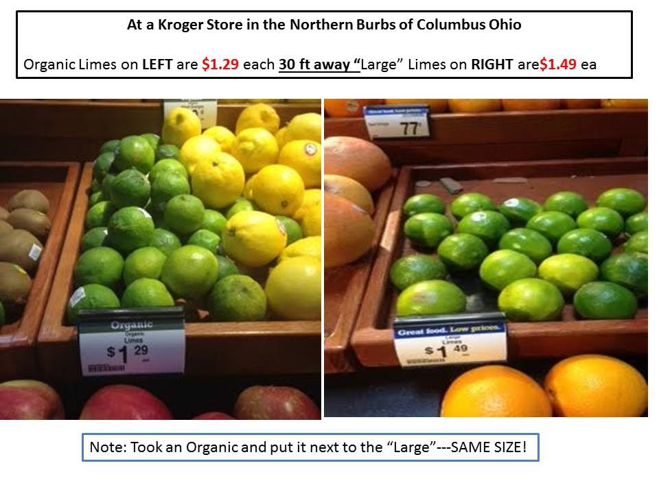
Price of Limes--Part 3. Are "Large Limes" and "Organic Limes" perfect substitutes for each other? And what is up with the pricing?

I guess limes have been my obsession lately.  Intrigued how Mexican criminal cartels are having an influence on the price of them.  Does not seem to be very "gang-like" to answer the question "What are you in for?" and have to admit you are in the illicit lime trade.

Well, anyway, I noticed this today. Organic limes are $1.29 and regular limes are $1.49.  Both within sight of each other. Both similar in size (I did a side by side comparison).

Usually the price differential is the other way around.

Oh, well.  Here is your brief Microeconomics lesson:

The "Substitution Effect" prompts movement up and to the LEFT along the Demand Curve for Large Limes as the Quantity Demanded decreases at $1.49 and the availability of a Substitute (Organic Limes) shifts the Demand Curve of Organic Limes to the RIGHT--at some price ($1.29) the Quantity Demanded is greater than it was before.

Top 10 Oil Producing Countries (including 1 US State that wants to be its own country!) in the World.

Interesting data (Carpe Diem at AEI) I think most Americans are unaware of.   Here is a list of the Top 10 oil producers in the world. I think most people would not put Russia at the top of the list and I don't think most would put the US at number 3.

Notice the insertion of Texas at number 8. If Texas were its own country (that is another subject!) it would rank number 8 in the world in oil output.  Texas alone produces 36% of the USA's oil production (2,826/7,864 X 100).

Even though the US is a dominant producer of crude oil, we still have to import it from foreign sources.

Source: AEI Carpe Diem

Looking at the list, can you guess which country the USA gets a majority of its imported oil?

Click below the fold to find out.

A new research paper on the "Amazon.com Tax". LOTS of lessons for Microeconomics!

Via Business Insider, THIS LINK is to a paper that researched the effect that levying State Sales Taxes on online purchases from Amazon.com. The results are an Economics teachers dream!  There are MANY basic microeconomics concepts explicitly discussed and illustrated.

This from the conclusion:

Internet taxation is an important issue that will continue to be debated for years to come.
Despite the importance of widespread “Amazon Tax” laws, little is currently known about their
effect on the demand for Internet retailers such as Amazon.com and whether the implementation of such laws leads to substitution effects such as bolstering local sales at brick-and-mortar stores when online retailers’ sales tax price advantage is removed.  

Using transaction-level data of 1.4 million households, we identify the effects of Amazon 
Taxes on the purchasing behavior of residents living in five states that adopted such laws over 
2012–2013. We find that Amazon sales fall by 9.5% after implementation of an Amazon Tax, corresponding to an elasticity of –1.3. We find the effect to be more concentrated in large purchases, such as those over $300. For this subset of purchases, we find that Amazon sales fall by 23.8% after implementation of the Amazon Tax, corresponding to an elasticity of –3.2.

I see an opportunity to learn the Substitution Effect, availability of Substitutes, elasticity of demand, incidence of taxation and who bears the burden of the tax, and Dead Weight Loss as the result of taxation.  A veritable cornucopia!! :)

The tax raises the price of the good BUT not by the full amount of the tax, dependent upon relative elasticities between buyers and sellers.  Because consumers are price sensitive (elasticity of 1.3) they decrease their Quantity Demanded (Point "A" to Point "B" along the "D*") because they have other online options with no sales taxes collected ("Substitution Effect").

The new Market Quantity will be at "Q1", less than it was prior to the tax.  So, solely due to the levying of the Sales Tax, Dead Weight Loss was created.  This means that there is a quantity of the good consumers don't get to enjoy at a lower price (area of Demand Curve represented by BLUE Triangle) and there is a quantity of the good that Amazon does not get to supply at a higher price (Red Triangle).

Notice the RED triangle is larger than the BLUE one.  This means that Amazon will bear a larger portion of the tax and will not be able to fully pass it on to the consumer. If they did, it would make things much worse for them. Consumers would move further UP and to the LEFT on the Demand curve, making the quantity sold even lower.

Chipotle and Marginal Revenue Product of Labor (MRP(L)). My two favorite things in one blog entry. Life is good (with a side of guac)..

Here is a nice real-life example using Chipolte to illustrate the AP Microeconomics concept of "Marginal Revenue Product of Labor (MRP L)".

Calculating MRPL is important in determining how many workers a firm should hire.

MRPL is obtained by multiplying Marginal Product ("MP") times the Price ("P") of the Good or Service.

Marginal Product is the physical amount of production EACH worker adds to the total.

So if a worker produces 10 units of a good (their "Marginal Product (MP)") and the price of the good is $1.00 then the Marginal Revenue Product of that workers Labor (MRPL) is $10.00.

Assuming Labor is the only input, a firm will hire up to the point where "MRP of Labor = Marginal Resource Cost (MRC)".  MRC is a fancy way of saying "Wage".  The MOST I am willing to pay this worker is $10.00 per hour.

Chipotle continues to refine the science of burrito velocity

Over the first three months of 2014, the US Mexican-food chain saw an average increase of seven transactions per hour at both peak lunch and dinner hours—12 to 1pm and 6 to 7pm, respectively. On Fridays, one of its busiest days of the week, Chipotle fielded 11 more customers per hour at lunchtime on average across its stores, a roughly 10% increase.

Chipolte has increased productivity on the burrito assembly line. Through efficiencies they have increased the number of transactions per hour.

This suggests that the Marginal Product of Labor for each worker has increased. Using my simple example above, if we increased productivity 10% then my worker now produces 11 units of the good.  If the price stays the same then the MRPL is now $11.00 (11 units of the good times $1.00).

Now, the firm faces a choice.

(1) It could hire an additional worker with the additional revenue and make life easier for the existing workers (this is what it could do if it operated in a "perfectly competitive labor market") .

(2) It could hire additional workers AND give raises to existing workers who increased the productivity by working more efficiently (this is what it would do if it operative in a "Monopsony labor market"".

(3) It could keep current staffing and wage levels and use the additional profit to open new stores. This would require additional workers to be hired, either at the same wages OR could be more (but likely not).

(4)It could keep the profits and stay at the status quo.

Looking at Chipolte's growth, I think they are pursuing #3.  They already pay above minimum wage so any increases in productivity seem to help fuel expansion with perhaps a side of wage growth on the side.

I could be wrong here.  I welcome alternative scenarios I may have missed. Thanks.  :)

AP Macroeconomics test hint: You must get "Employment" and "Unemployment" right when asked how it changes as the result of a Real GDP change.

I know this is VERY EASY but lots of students get it wrong, mostly because of inattention and/or nerves while taking the test.  Don't miss this EASY point!

My cyber-friend over at The New Arthurian has this graph showing the relationship between POSITIVE relationship between Real GDP and Employment (the relationship is NEGATIVE between Real GDP and UN-employment)

All the lines show the percentage change in that variable year-over-year.  Real GDP is in BLACK and the other measures of EMPLOYMENT are in the the various other colors.

The New Arthurian

Below is the same graph (but starting in 1950) but with only with the change in Real GDP and "Total Non-Farm Employment" to simplify the visual.

Notice the trend?  Real GDP(BLACK line) "pulls up"  or "pushes down" employment.

If you have a question on the AP Macroeconomics test that asks how employment is affected as a result of and INCREASE in Aggregate Demand (AD) OR an increase in Aggregate Supply (SRAS or LRAS) you would answer like this:

"As Real GDP (output) increases business need more workers to produce the additional goods and/or services.  More labor is needed and the EMPLOYMENT Rate will INCREASE.

If the question asks how employment is affected as a result of a DECREASE in Aggregate Demand (AD) or a DECREASE in Aggregate Supply (SRAS or LRAS) you would answer like this:

"As Real RDP (output) decreases businesses will need fewer workers because they are producing fewer goods and/or services. Less labor is needed and the EMPLOYMENT rate will DECREASE".

The graph below illustrated the NEGATIVE or INVERSE relationship between Real GDP and the UN-employment rate---the number of people without jobs but are actively seeking one.

As the Real GDP Increases the UNEMPLOYMENT rate DECREASES.

If you have a question on the AP Macroeconomics test that asks how unemployment is affected as a result of an INCREASE in Aggregate Demand (AD) OR an increase in Aggregate Supply (SRAS or LRAS) you would answer like this:

"As Real GDP (output) increases business need more workers to produce the additional goods and/or services.  More labor is needed and the UNEMPLOYMENT Rate will DECREASE.

If the question asks how employment is affected as a result of a DECREASE in Aggregate Demand (AD) or a DECREASE in Aggregate Supply (SRAS or LRAS) you would answer like this:

"As Real RDP (output) decreases businesses will need fewer workers because they are producing fewer goods and/or services. Less labor is needed and the UNEMPLOYMENT rate will INCREASE".

Read those answers in BOLD again so you fully understand how to answer a question when asked how EMPLOYMENT or UNEMPLOYMENT is affected by a change in Real GDP.  While they both indicate the same thing (an improving or declining economy) , the directional change in important for you to get right on the test.

A small thing, I know, but it WILL cost you a point if you don't get the terminology right.

"Too much money chasing too few dinners". Food prices are not rising because of Monetary Policy. Think Supply and Demand fundamentals instead

The prices of wide swaths of food items have increased over a relatively short period of time.  The longer term trend in rising prices has been the increased demand from developing countries, China being the most notable.  As disposable incomes increase people (1) consume more food overall and (2) become more diverse in what they consume (more meat and a variety of veggies along with grains already consumed).

When quantity demanded is greater than quantity supplied, over time prices inevitably rise.

Short term variables, like weather and disease (plant and animal), affect harvests and the stockyards in the interim.  This combination seems to be prevailing force behind the rise in prices at the grocery store.

One distinction I would like to make is "food inflation" is not a product of Monetary policy and the excessive "printing of money".  It is a product of market fundamentals mentioned above--the push (supply side) and pull (demand side) of Supply and Demand.

It is a scarcity of output/production as opposed to an abundance of money that is the primary cause of rising food prices we have seen as of late.

Here is a list from USA Today of 10 food items that have increased in price in the short and long(er) term.

1. Bacon
> 4-yr. change: +53%
> 1-yr. change: +13%
> Current price: $5.55 per lb.

2. Ground Beef
> 4-yr. change: +35%
> 1-yr. change: +8%
> Current price: $4.13 per lb.


3. Oranges
> 4-yr. change: +35%
> 1-yr. change: +23%
> Current price: $1.21 per lb.


4. Coffee
> 4-yr. change: +31%
> 1-yr. change: -17%
> Current price: $5.00 per lb.